Derrick Burt's GIS Portfolio
A collection of GIS analyses and maps.
Evaluating Reproducibility and Replicability of GIS Vulnerability Analysis
Background
Reproducibility and replicability of scientific research is becoming more widely recognized as an essential component of a robust scientific method in academic research. The National Academies of Sciences, Engineering, and Medicine defines and differenaties the two as such: reproducibility aims to obtain the same results by using the same input data and methodology while replicability aims to answer the same question using different different data and similar methodologies (2019). Adopting these processes in scientific research not only allows for a greater scrutiny of one’s methodology but opens up new avenues of communication and transparency between researchers. Reproduciblity and replicabiltiy are instric to an open-science that not only allows for self-correction but sees it as beneficial to the scentific community as a whole (Sui 2014).
Applying these practices to climate change vulnerability research can be complicated by the confusion that surrounds vulnerability as a theoretical concept. Climate vulnerability is highly complex, contextual, and place-specific which makes it difficult to scale or replicate (Hinkel 2010). As a result of this, it is difficult for researchers and policy makers to agree upon a central, uniform approach to studying climmate vulnerability. Defining vulnerability not as an observable event but instead as a theoretical framework, Hinkel identifies the importance of developing an ‘operational definition,’ or a framing methodology, of any given vulernability analysis (2010). Using this framework, Hinkel encourages a critical engagement and interrogation of the methodological approaches used in vulnerability analyses.
Purpose
The goal of this exercise is to reproduce and evaluate the methodologies Malcomb et al. has used to define and visualize climate vulnerability in Malawi. First, we will examine the methodology of Malcomb et al.’s analysis and use it to reproduce Figure 4 and Figure 5 from the research paper. Then, we will reflect upon the authors’ methodological approach, bringing in literature on vulnerability analysis.
Malcomb et al. Methodology for Household Resilience in Malawi
Goal
In their paper, Malcomb, Weaver, and Krakowka outline a new approach to modelling climate vulnerability in sub-Saharan Africa. Their vulnerability model employs a ‘multi-scale, multi-indicator’ approach to household-level climate vulnerability with the goal of providing both local actors and policy makers the ability to identify high risk areas and possibly solutions. They claim that their approach is both scalable and flexible so that it can be employed by other countries within sub-Saharan Africa.
Methodology
Malcomb et al. use a multi-criteria weighted analysis to analyze and visualize social, economic, cultural, and environmental vulnerability indicators. These vulnerability indicators were divided into three sub-categories: adaptive capacity (composed of both assets and access), livelihood sensitivity, and physical exposure. Each of these vulnerability indicators were rescaled into quintiles: a 0 (worst) to 5 (best) scoring system. The authors used the following weighting scheme to produce a household resilience score for each Traditional Authority (TA: the scale of analysis, an administrative boundary just below districts): Household Resilence = Adaptive Capacity(.4) + Livelihood Sensitivity(.2) + Physical Exposure (.2).

Reproducing Malcomb’s Methodology and Figures
Software
The following softwares were used to complete this exercise:
Data
We used the following data to reproduce Malcomb et al.’s methodology:
- DHS Malawi Household Surveys: Access to this data requires an account and a formal request based on project
- DHS Cluster Points: Household groupings where surveys were collected
- DHS Survey Boundaries
- Flood and Drought Rasters from UNEP GLobal Risk Data Platform
- Livelihood Zones from FEWSnet
- Traditional Authority Shapefile: Gathered from GADM
- OSM Malawi Lakes from MASDAP
- National Parks from Protected Planet
Calculating Adapative Capacity Scores (Fig 4)
To get the DHS data into a PostGIS database, we used this R script written by Professor Holler. This script is meant to write SPSS files into a Postgres database, so be sure to downlaod the DHS data as an SPSS file (if you have access).
The following sql code was written to convert the DHS household criteria into composite capacity scores. I will provide a commented walk-through of the code and emphasize areas that problematize the reproducibility Malcomb et al.’s methodology
Identify urban areas from DHS clusters and join to DHS survey data:
/* codes
household id: hhid
cluster id:
livestock: HV246a + hv246a + hv246d + hv246e + hv246g
sick: hv248
land: hv245
wealth: hv271, or should it have been hv270 (already on scale of 5?)
orphans: hv251
watertime: hv204
electricity: hv206
cookingfuel: hv226
gender: hv219
cellphone: hv243a
radio: hv207
urban: joined from DHS clusters
*/

/* Identify the TA each cluster is in to find which clusters are urban or rural and join to dhs table */
update mwita set geom =
st_makevalid(geom)
where not st_isvalid(geom)

alter table dhsclusters add column ta_id integer;
update dhsclusters set ta_id = mwita.id from mwita where st_intersects(mwita.geom, dhsclusters.geom);

select count(name2_), count(distinct name2_) from mwita;
--the TA names are not unique! Use the ID instead...

alter table dhshh1010 add column ta_id integer;
update dhshh1010 set ta_id = dhsclusters.ta_id from dhsclusters where dhsclusters.dhsclust = dhshh1010.hv001;

alter table dhshh10 add column urbanrural varchar(1);
update dhshh10 set urbanrural = dhsclusters.urban_rura from dhsclusters where dhsclusters.dhsclust = dhshh10.hv001;

create table mwi as
select st_union(st_makevalid(geom))::geometry('multipolygon',4326) from mwita;
Get rid of null values or missing data:
--originally having 24825 records
DELETE FROM dhshh1010 WHERE
hv246a=98 or
hv246a=99 or
hv246d=98 or
hv246d=99 or
hv246e=98 or
hv246e=99 or
hv246g=98 or
hv246g=99 or
hv219=9 or
hv243a=9 or
hv245=99 or
hv206=9 or
hv204=999 or
hv204=998 or
hv226=99 or		 --no cooking data
hv226=95 or 	    --no cooking
hv226=96 or		   --cooking with 'other' fuel
HV207=9;
/*deleted 156 household records with missing data for our purposes
resulting in ## records*/
Combine different livestock into one column and show with percent rank:
/*count livestock*/
ALTER TABLE dhshh1010 ADD COLUMN hhlivestock INTEGER;
UPDATE dhshh1010 SET hhlivestock = hv246a + hv246d + hv246e + hv246g;

/*illustrate with percent_rank() and ntile()*/
select hhlivestock,
(percent_rank() OVER(ORDER BY hhlivestock asc) * 4) + 1 as pctRtimes4plus1,
percent_rank() OVER(ORDER BY hhlivestock asc) as pctRank,
ntile(5) over(order by hhlivestock asc) as ntile5
from
dhshh1010
Here is a small subset of our code to convert the household level data to quintiles. This was one of the more difficult portions of the methodology to reproduce. While Malcomb et al. explains that they reclassified these sets of data into quntiles from 0 to 5 (notwithstanding the fact that 0 to 5 actually represents 6 classes), they did not explain in detail the decision making processes that went into these classifications.Further, 5 of the 12 household variables were represented either a 0 or 1 score, and there was no explanation as to how these variables were weighted nor any justification for the decision to use quintiles.
/* Standardizing to scale of 1 (low capacity) to 5 (high capacity) */
/*  ORDER BY DESC will make high values to recieve a low score
	ORDER BY ASC will make low values to receive a low score  */

ALTER TABLE dhshh10 ADD COLUMN livestock REAL;
UPDATE dhshh1010 set livestock = pctr FROM
(SELECT hhid as shhid, percent_rank() OVER(ORDER BY hhlivestock asc) * 4 + 1 as pctr FROM dhshh10 ) as subq
where hhid=shhid;

ALTER TABLE dhshh1010 ADD COLUMN sick REAL;
UPDATE dhshh1010 set sick=pctr from
(SELECT hhid as shhid, percent_rank() OVER(ORDER BY hv248 desc) * 4 + 1 as pctr FROM dhshh10 ) as subq
where hhid=shhid;
--ORDER THIS DESC because if MANY people were sick they need a LOW capacity score

ALTER TABLE dhshh1010 ADD COLUMN land REAL;
UPDATE dhshh1010 set land=pctr from
(SELECT hhid as shhid, percent_rank() OVER(ORDER BY hv245 asc) * 4 + 1 as pctr FROM dhshh10 ) as subq
where hhid=shhid;
--See code to observe how the rest of the non-binary variables were reclassified

/* The following code shows how the binary (0 or 1) variables were given their scores */
ALTER TABLE dhshh10 ADD COLUMN sexcat REAL;
UPDATE dhshh10 set sexcat=
	CASE
		WHEN hv219 = 1 THEN 5
		ELSE 1
	END;

ALTER TABLE dhshh10 ADD COLUMN cellphone REAL;
UPDATE dhshh10 set cellphone=
	CASE
		WHEN hv243a = 1 THEN 5
		ELSE 1
	END;

ALTER TABLE dhshh10 ADD COLUMN radio REAL;
UPDATE dhshh10 set radio=
	CASE
		WHEN hv207 = 1 THEN 5
		ELSE 1
	END;

ALTER TABLE dhshh10 ADD COLUMN urbanruralscore REAL;
UPDATE dhshh10 set urbanruralscore =
	CASE
		WHEN urbanrural = 'U' THEN 4
		ELSE 3
	END;
From here, the scores were weighted from a scale of .4 to 2.0 scale so that the final household resilience calculation (including the other elements) would scale from 0 to 5.
/* Create a composite household capacity score, on scale from 0.4 to 2 */
ALTER TABLE dhshh10 ADD COLUMN capacity REAL;
UPDATE dhshh10 SET capacity =
(livestock*0.04+
sick*0.03+
land*0.06+
wealth*0.04+
orphans*0.03+
water*0.04+
electricity*0.03+
cooking*0.02+
sexcat*0.02+
cellphone*0.04+
radio*0.03+
urbanruralscore*0.02);

CREATE VIEW tacapacity AS
SELECT ta_id, count(capacity) as hhcount, avg(capacity) as capacityavg, min(capacity) as capacitymin, max(capacity) as capacitymax, stddev(capacity) as capacitystddev
FROM dhshh10
GROUP BY ta_id;

ALTER TABLE mwita ADD COLUMN capacity REAL;
UPDATE mwita SET capacity = capacityavg
FROM tacapacity
WHERE tacapacity.ta_id = mwita.id

CREATE TABLE capacity AS
SELECT ST_AsRaster(mwita.geom, (select rast from drought limit 1), '32BF', mwita.capacity, -9999) as rast
FROM mwita
where capacity is not null
Calculating Sensitivity
We could not calculate the livelihood sensitivity scores (from FEWSnet) because this data is no longer available. This means 20% of our final household resilience score is missing if we compare to Malcomb’s.
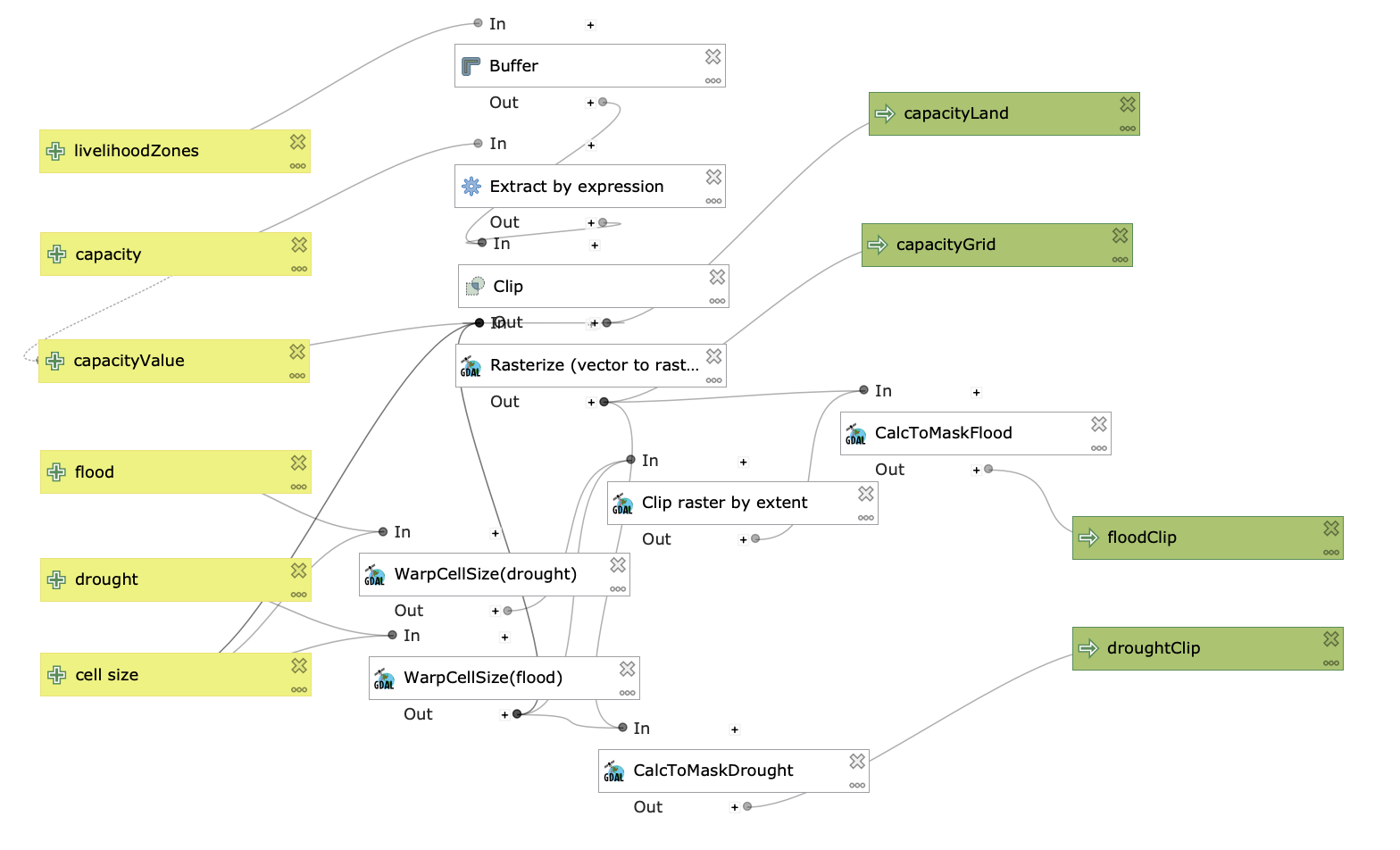
Calculating Physical Exposure with GRASS Tools and QGIS Model Builder
We performed the raster calculations with with QGIS model builder and GRASS tools in QGIS instead of using PostgreSQL. It is possible to load raster data into a postgres database with raster2pgsql (if you have installed postgis with homebrew, it will already be on your computer). We used model builder to allow us to clip, reproject, and resample our two input rasters (drought and flood) and rasterize our adaptive capacity scores to allow for a final calculation.
The model, modified from an original version constructed by Professor Holler, does the following:
*(Refer to this image of the model for a visual aid.)
- Takes the adapative capacity scores, uses
extract by expressionto remove null values, and useclipto crop by livelihood zones to produce capacityLand - Takes the adaptive capacity scores, uses
extract by expressionto remove null values, and usesrasterizeto produce capacityGrid (this rasterized layer will be used to clip other rasters) - Adds a ‘cell size’ input so that the user can choose a cell size (the default is 0.041667 decimal degrees, or 2.5m)
- Takes the flood layer, uses
warp cell sizeto change cell size based on the input, then masks the layer by capacityGrid to produce floopClip - Takes the flood layer, uses
warp cell sizeto change cell size based on the input, then masks the layer by capacityGrid to produce droughtClip
After this step, we are almost ready to calculate the three rasters to get a final raster of the household resilience scores, but we first need to recalculate the flood and drought rasters into quintiles. The floodClip layer is already on a 0 to 4 scale, and can be converted to a 1 to 5 scale in raster calculator. The drought clip can be reclassified with GRASS tools using two steps:
- Input the layer into
r.quantileusing these paramaters: be sure to check the “generate recode rules…” box and output the file as a .html - Input the drought layer in
r.recodeusing the .html output as the “File containing recode rules”
Combining Indicators to Calculate Final Resilience Score (Fig. 5)
With the three rasters properly clipped and classified, the following calculation in raster calculator was made to reproduce Figure 5:
((2- capacityGrid@1)*(.4) + (droughtRecode@1)*(.2)) + ((floodClip25@1)*(.2))
Results
Figure 4
This is my replication of Figure 4. Despite being created from the same exact data, It has not been reproduced exactly as the variables are scored with a different scale and show different geographic patterns in vulnerability.
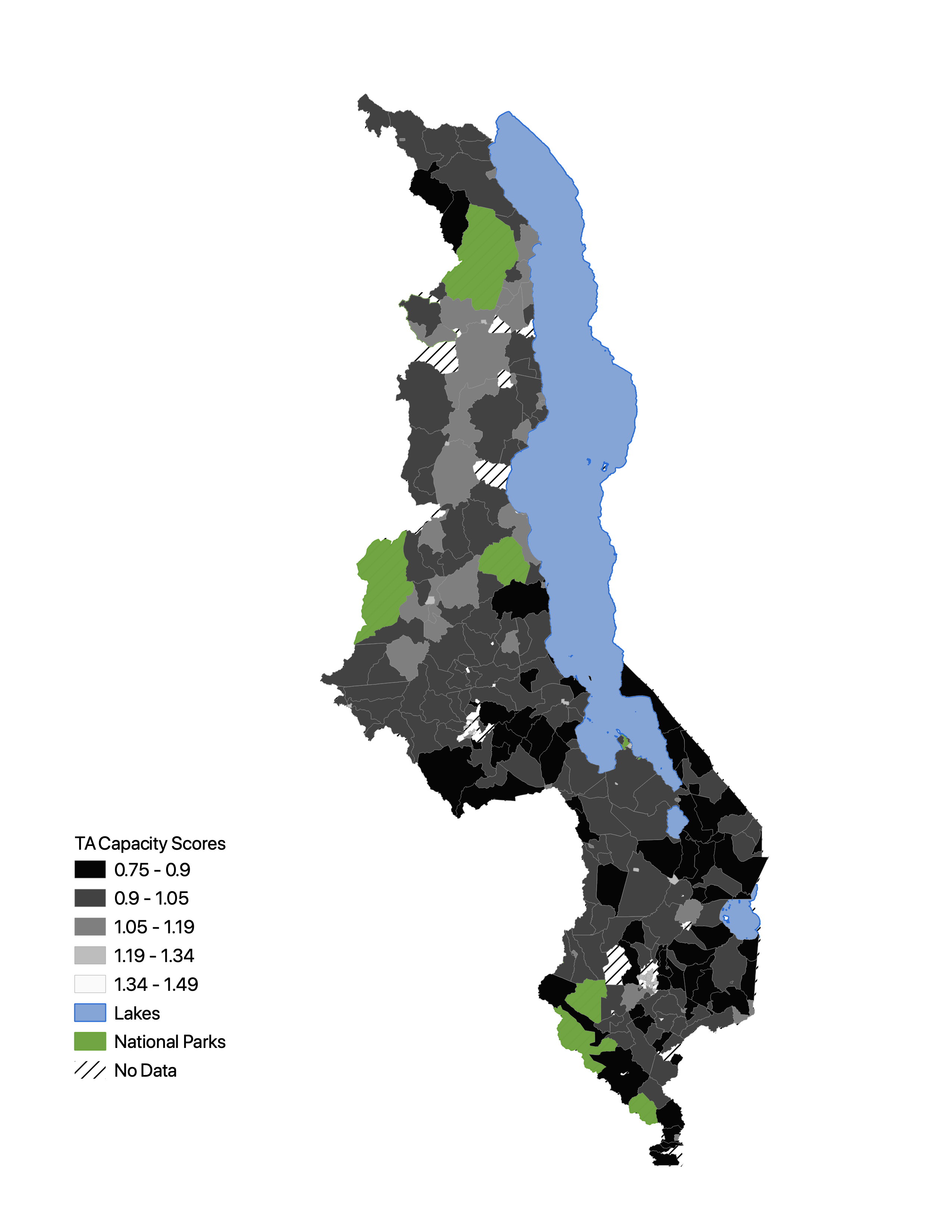
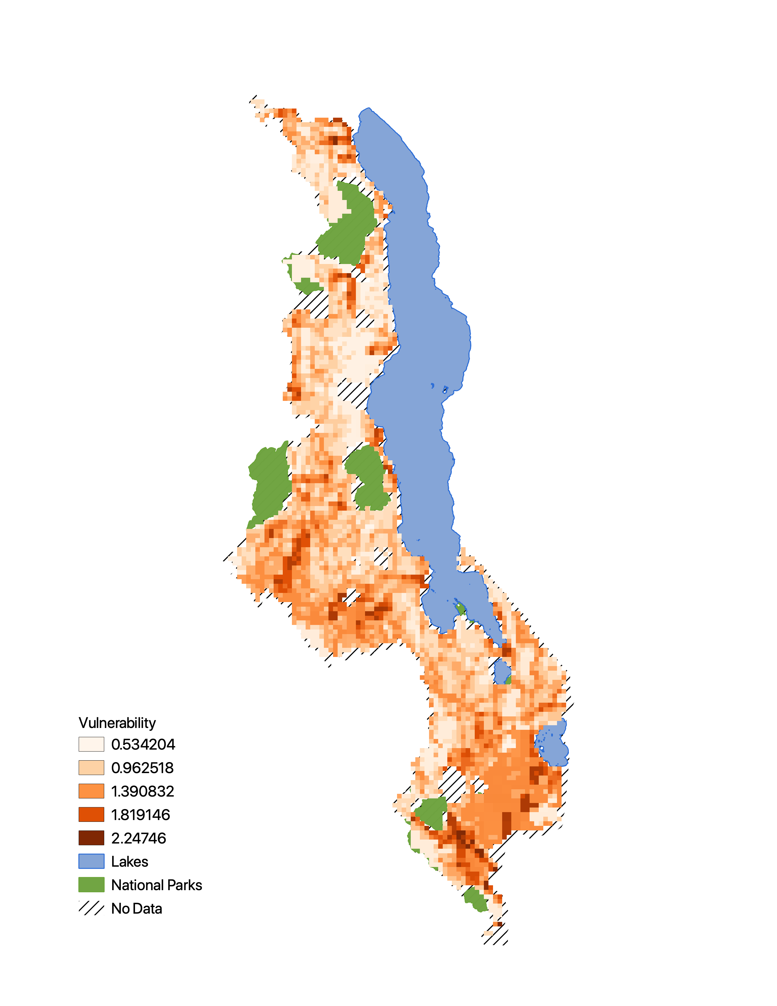
Figure 5
This is my replication of Figure 5. It is missing 20% of the Malcomb calculation, and given the difference in our DHS survey quintiles from Figure 4, that is also skewing our results from theirs.
Discussion
Both of the figures we attempted to produce have some notable distinctions from those published in Malcomb et al. Our reproduction of Figure 4, depsite having the same exact data and attempting to replicate the bits of their methodology that was explained, have neither the same range of scores nor the same distribution of capacity scores. Our also has larger clusters of more vulnerable (lower capacity) TAs in central Malawi. Figure 5, even if we were able to incorporate the FEWSnet sensitivity data, is also skewed by our results from the household scores. Even though we can see similar vulnerability patterns in the south and central regions, most of the northern porition of our figure is quite different from that of Malcomb’s.
Although the authors’ claim they employ a “transparent and easily replicable methodlogy” in this study (Malcomb et al. 2014), I argue that this research is not reproducible. While policy makers and local actors in sub-Saharan Africa might be able to borrow the author’s framework of using multi-criteria vulnerability indicators to visualize climmate capacity, we could not reproduce the results of this research using the same inputs to yield the same outputs (National Academies of Sciences, Engineering, and Medicine 2019). The impediments to this paper’s reproducibility may be explained by the authors’ incomplete or limited sharing of their methodology, the complexity of climate vulnerability analyses, as well as the general structure of academic research that does not allow for publications, as well as their methods and research, to be updated (Sui 2014). I will examine some of the components that prevent this research from being fully reproducible.
First, because we were missing all of the FEWSnet sensitivity data, we would have only been able to produce 80% of the authors’ final results. This cannot be seen as an error on the part of the authorship, but we might rather intrepret this as a shortcoming of the institutional structures of geographic publishing. If there were to be a true community that supported open publication, then perhaps the industry itself could provide an archival network of any relevant data needed to reproduce any given study (Sui 2014).
Even if we had been able to acquire all the relevant data, there were still holes in the methods section that left us in the dark when it came to understanding important decision-making in the data analysis process. Perhaps the most notable issue here was in the reclassifying of the DHS household capacity indicators. Although the author’s explained that they did reclassify, they did not specify exactly how, which became especially confusing when we tried to reclassify the binary indicators. Explaining these decision making processes is a crucial component of robust research for two reasons. First, it allows for a scrutinuous and exact reproduction of the research that enables a greater understanding of the decisions. Second, when “index developers are faced with choices between plausible alternatives, (they introduce) subjectivity into the modeling process… (and) changes in input data and algorithms have the potential to significantly influence the output” (Tate 2012). Therefore, we can both reproduce the work and understand the subjectivity that went into the decision making and articulate possible limitations.
Further, there is an insufficient acknowledgement or quantifiable measurements of error in the authors’ analysis. Without fully explaining the rationale behind their choice of indicator variables, the authors don’t leave room to acknowledge possible sources of bias in their decision making structure, which is an essential component when measuring something as subjective as social vulnerability (Tate 2014). Further, they fail to include a summary statistics of their survey data, making their sample size, the presence of outliers, etc. unclear (Tate 2014). Without accounting for any modifications, or lack thereof, that were made to the data before the analysis, makes it difficult to sturdily reproduce or interrogate the research.
The process of attempting to reproduce these two figures emphasizes the value in a comprehensive accounting of any research-based methodological approach. Although the publication allows us to employ a similar methodology, we cannot reproduce their own and therefore cannot strictly scrutinize some of the subjective decision-making or possibility for error in this analysis. Without acknowledging these subjectivities, readers and, more detrimentally, policy makers can be mislead and regions can be misrepresented. It is possible that, with a more thorough account of the methodology, we would be able to more accurately reproduce, understand, and critque this multi-scale and multi-criteria vulnerability analysis. However, we should also recognize the impediments to reproducibility and replicability that seem to exceed (or perhaps precede) the authors. First, the nature of the academic publishing industry does not support an archive of easily-accessible data for reproducing research. Second, vulnerability is a commplex and immeasureable phenomenona that cannot be easily replicated or scaled. Thus, while we there are identifiable impedimemnts to reproducibility in Malcomb et al.’s methodology, the field of publishing reproducible and replicable climate vulnerability research presents its own difficulties.
Resources
Hinkel, J. (2011). “Indicators of vulnerability and adaptive capacity”: towards a clarification of the science–policy interface. Global Environmental Change, 21(1), 198-208. https://doi.org/10.1016/j.gloenvcha.2010.08.002
Malcomb, D. W., Weaver, E. A., & Krakowka, A. R. (2014). Vulnerability modeling for sub-Saharan Africa: An operationalized approach in Malawi. Applied geography, 48, 17-30. https://doi.org/10.1016/j.apgeog.2014.01.004
National Academies of Sciences, Engineering, and Medicine. 2019. Reproducibility and Replicability in Science. Washington, DC: The National Academies Press. doi: https://doi.org/10.17226/25303.
Sui, D. 2014. Opportunities and impediments for Open GIS. Transactions in GIS, 18(1); 1-24. doi: 10.1111/tgis.12075
Tate, E. (2012). Social vulnerability indices: a comparative assessment using uncertainty and sensitivity analysis. Natural Hazards, 63(2), 325-347. https://doi.org/10.1007/s11069-012-0152-2,