Derrick Burt's GIS Portfolio
A collection of GIS analyses and maps.
Replicating CyberGISX Analysis: Rapidly Measuring Spatial Accessibility of COVID-19 Healthcare in Connecticut
About
In their paper, “Rapidly Measuring Spatial Accessibility of COVID-19 Healthcare Resources: A Case Study of Illinois, USA”, Kang et al. implement a methodology that measures and visualizes the access that two different populations, COVID-19 patients and the population risk (defined as those over 50), have to two important resources, ICU beds and Ventilators.
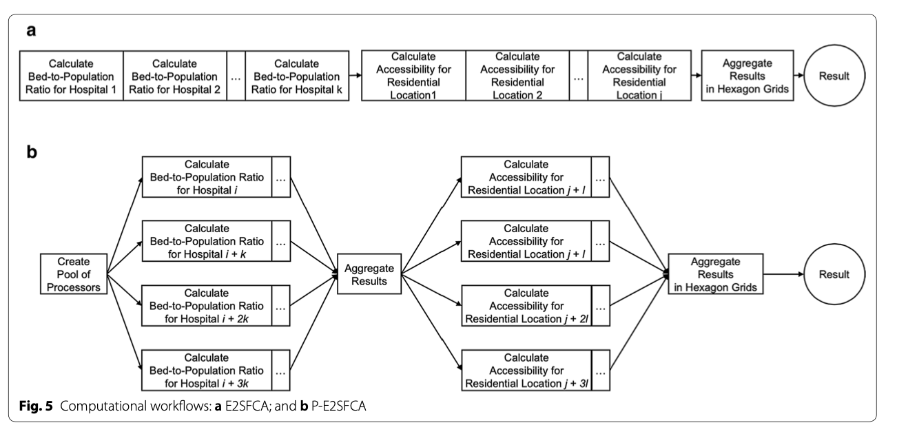
To rapidly measure accessibility to Covid-19 healthcare, Kang et al. developed a methodology for parallel implementation of an Enhanced Two-Step Floating Catchment Area (E2FSCA) methodology. This method calculates the ratio between a service (in this scenario, hospital ICU beds or ventilators) and the population in its surrounding area, accounting for distance decay. Because this is a computationally intensive analysis hat uses large street networks, the authors developed a parallel-E2FSCA (P-E2FSCA), which enables the use of up to 4 processors while implementing the analysis.
The following resources document their methodology, data, and results:
- Paper: an overview of the problem, description of conceptual methodology and analysis, results, and conclusion
- Jupyter Notebook: a reproducible implementation of the paper’s methodology (requires a CyberGISX account)
- Github Repository: has the notebook and all the necessary data
- Where COVID-19 Spatial Access Dashboard: A live dashboard that displays the daily accessibility calculated from this methodology
Purpose
The purpose of this exercise is to replicate Kang et al’s methodology, using a Jupyter Notebook on their CyberGISX platform, to calculate spatial accessibility of COVID-19 healthcare resources in Connecticut. I will briefly summarize their methodology, walk through the process of acquiring and processing the necessary data for Connecticut, show and explain the code modifications that were made to Kang et al’s Notebook for this replication, explain the results, and comment on the methodology and the process of replication.
Important:
- Most of the code is an exact replication of Kang et al.’s methodology (unless explicitly noted, it should be assumed that any code was written by Kang et al.)
- Note on reproducibility: the notebook was run in the CyberGISX environment, so even with the data and notebook provided, my replication is only exactly reproducible within the CyberGISX platform. Otherwise, you will need to install all of the python packages on your local jupyter platform, and then the notebook should work.
Kang et al. Methodology
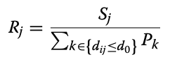
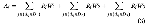
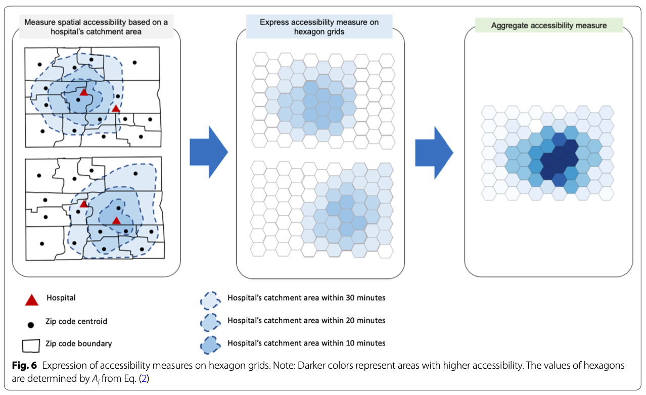
To the measure spatial accessibility of COVID-19 healthcare resources, Kang et al. use a P-E2SFCA. Essentially, their two-step methodology first finds the size of the population (of either COVID-19 patients or population over fifty) within staggered catchment areas of hospitals. They do this by locating the nearest node on Open Street Map network (specifically using OSMNX, a python package to import OSM networks) to each hospital, and calculating catchment areas of 10, 20, and 30 minute drive times whose precise network sizes are determined computationally by creating convex hulls. The population of a catchment area is found by locating the centroids of the population’s given geography (for covid, zip code level, and for over fifty, census tracts) within the catchment area. After the catchment areas are calculated, a service-to-population ratio is calculated to find the available resources (ICU beds or Ventilators) to the desired population. To allow for comparison, an accessibility measurment is created to normalize the results. These accessibility measures are mapped onto hexagonal grids, and then aggregated into one hexagonal grid, measuring accessibility on a relative scale of 0 to 1 (1 being the relatively most accessible, 0 being relatively least). More accessible areas will be those with the most overlapping catchment areas with more available resources (clusters of hospitals with more resources). This workflow is implemented in a parallel fashion, splitting up the computational processing between 1, 2, 3, or 4 processors (based on user’s choice).
These accessibility measurements produce 4 outputs: At Risk population’s access to ventilators, Covid patients access to ventilators, At Risk population’s access to ICU beds, Covid patients access to ICU beds. This analysis is done for both Chicago as well as the entire state of Illinois.
This figure, from the paper, provides a conceptual workflow of the spatial analysis:
This figure, from the paper, provides a conceptual workflow of the parallel computation:
Additionally, the authors compare the Social Vulnerability Index in high and low accessibility areas. This portion of the analysis is not included in the Jupyter notebook.
Replicating the Notebook for Connecticut
I have attempted to replicate Kang et al.’s methodology for the State of Connecticut. The following steps outline the process of gathering the data, preparing it for analysis, tweaking the notebook, and the results. Most of the analysis follows Kang et al’s methodology, but here are some important deviations my replication has taken from their analysis:
- I only examine accessibility at the state level for Connecticut
- There was no available ventilator data for CT, so I examine accessibility to ICU beds and total beds
- I include hospitals in RI, MA, and NY that are within 15km buffer of the CT border, to account for CT residents that may cross state lines for COVID care
Software
The following software was used in the analysis:
Data and Notebook
The following data was used for the analysis, all of the shapefiles can be downloaded from this geopackage:
- Hospital Shapefile and Bed Data from HIFLD Open Geoplatform
- ICU Beds from the Department of Health
- CT Census Tract Boundaries from Census Bureau
- CT Census Tract Population by Age from Census Burearu
- CT Active Covid Cases by Town (11/15/20-11/28/20) from CT Open Data Portal
- Town Shapefile from CT Open Geodata Portal
The final version of my notebook can be downloaded here - If you are not running on CyberGISX platform, you must install all libraries in the first code cell.
Preparing the Data
The Hospital shapefile data was brought into QGIS prepared with the following steps:
- Draw a 15km buffer around state (‘ctState’ in geopackage):
Processing Toolbox > Buffer > parameters: input layer: 'ctShapefile', distance: '15km', output: 'Buffered' - Extract hospitals the intersect are within buffer:
Processing Toolbox > Extract by Location > parameters: Extract features from: 'hospitals', where the features : 'intersect', 'are within', by comparing to features from: `Buffered`, output: 'hospitalsBuffered' - Eliminates duplicates (each hospital had a duplicate in attribute table):
Processing Toolbox > Delete duplicates by feature attribute > parameters: Input layer: `hospitalsBuffffered`, Fields to match duplicate by: `NAME`, output: hospitalsNoDup - Select only hospitals that are “GENERAL ACUTE CARE”:
Processing Toolbox > Extract by Expression > parameters: Input layer: 'hospitalsNoDup', Expression: "TYPE" = 'GENERAL ACUTE CARE', output:'hospitalsCToICU'
The ICU Bed data was brought into QGIS and cleaned with the following steps:
- Keep the first 13 fields (important hospital information) as well as ‘total_icu_beds_7_day_avg’ from hospitalsICU by navigating to:
Properties > Fields > Toggle editing mode > Delete Fieldsand deleting the undesired fields - Join hospital ICU data to hospital shapefile by address (somehow this worked, all 65 hospitals in both datasets had the same exact address:
Processing Toolbox > Join Attributes by Field Value > parameters: Input layer: 'hospitalsCT', Table field: `ADDRESS`, Input layer 2: 'hospitalsICU1`, Table field: `address`, Layer 2 fields to copy: 'ICU', Join type: 'one-to_one', output: 'hospitalsCT'
The Population data was cleaned in Excel (summing the population age groups (50-54….85+) into ‘OverFifty’ and then brought into QGIS as ‘popTracts’ and processed with te following step:
- Join the population over Fifty to the tracts:
Processing Toolbox > Join Attributes by Field Value > parameters: Input layer: 'tracts', Table field: `AFF_GEOID`, Input layer 2: 'popTracts`, Table field: `GEOID`, Layer 2 fields to copy: 'OverFifty', Join type: 'one-to_one', output: 'csTracts'
The Covid data was cleaned in QGIS with the follow step:
- Join the covid cases to the towns:
Processing Toolbox > Join Attributes by Field Value > parameters: Input layer: 'town', Table field: `Name`, Input layer 2: 'ctCovid`, Table field: `Name`, Layer 2 fields to copy: 'cases', Join type: 'one-to-one', output: 'covidTowns'
The hexagonal grid was processed in QGIS with the following step:
- Create a hexagonal from ‘ctState’:
Processing Toolbox > Create Grid > parameters: Grid type: 'hexagon', Grid extent: Use layer extent ('ctShape'), Horizontal spacing: 1.5km, Vertical spacing: 1.5km, Grid CRS: EPSG:32618, output: ctGrid
With all the necessary shapefiles prepared, the data were uploaded to the CyberGISX notebook.
Altering the Notebook
The following chunks of code were altered from Kang et al. to replicate the P-E2SFCA methodology for the state of Connecticut. Code is commented #DERRICK: where it was altered by myself and commented #JOE where altered by Professor Holler.
Load population data:
#DERRICK: change to CT over fifty by tracts
pop_data = gpd.read_file('./CTData/PopData/csTracts.shp')
pop_data.head()
Load covid data:
#DERRICK: change to CT covid by town
pop_data = gpd.read_file('./CTData/PopData/covidTown.shp')
pop_data.head()
Load hospital data:
#DERRICK: change to CT hospitals
hospitals = gpd.read_file('./CTData/HospitalData/hospitals.shp')
hospitals.head()
Map hospital data:
# DERRICK: switch lat long to CT, bring out starting zoom a bit
m = folium.Map(location=[41.5, -72.65], tiles='cartodbpositron', zoom_start=8.47)
for i in range(0, len(hospitals)):
folium.CircleMarker(
# DERRICK: add CT data, edit lat long and pop ups
location=[hospitals.iloc[i]['LATITUDE'], hospitals.iloc[i]['LONGITUDE']],
# getting error tuple index out of range
# popup="{}{}\n{}{}\n{}{}".format('Hospital Name: ',hospitals.iloc[i]['NAME']),
#'Beds: ',hospitals.iloc[i]['BEDS']),
radius=5,
color='grey',
fill=True,
fill_opacity=0.6,
legend_name = 'Hospitals'
).add_to(m)
legend_html = '''<div style="position: fixed; width: 20%; heigh: auto;
bottom: 10px; left: 10px;
solid grey; z-index:9999; font-size:14px;
"> Legend<br>'''
m
Load ct grid :
# change to CT grid file
grid_file = gpd.read_file('./CTData/GridFile/ctGrid.shp')
grid_file.plot(figsize=(8,8))
Load CT street network with 15km buffer :
#DERRICK: switch to CT and add buffer_dist
if not os.path.exists("CTData/CT_Buffered_Network.graphml"):
    G = osmnx.graph_from_place('Connecticut', buffer_dist=15000, network_type='drive')
    osmnx.save_graphml(G, 'CT_Buffered_Network.graphml', folder="CTData")
else:
    G = osmnx.load_graphml('CT_Buffered_Network.graphml', folder="CTData", node_type=str)
osmnx.plot_graph(G, fig_height=10)
Alter pop_centroid function for CT data :
# to estimate the centroids of census tract / county
def pop_centroid (pop_data, pop_type):
    pop_data = pop_data.to_crs({'init': 'epsg:4326'})
    if pop_type =="pop":
        pop_data=pop_data[pop_data['OverFifty']>=0]
    if pop_type =="covid":
        # DERRICK: change 'cases' to 'Cases'
        pop_data=pop_data[pop_data['Cases']>=0]
    pop_cent = pop_data.centroid # it make the polygon to the point without any other information
    pop_centroid = gpd.GeoDataFrame()
    i = 0
    for point in tqdm(pop_cent, desc='Pop Centroid File Setting', position=0):
        if pop_type== "pop":
            pop = pop_data.iloc[i]['OverFifty']
            # believe 'GEOID' will work
            code = pop_data.iloc[i]['GEOID']
        if pop_type =="covid":
            pop = pop_data.iloc[i]['Cases']
            # change ZCTA5CE10 to objectid
            code = pop_data.iloc[i].OBJECTID
        pop_centroid = pop_centroid.append({'code':code,'pop': pop,'geometry': point}, ignore_index=True)
        i = i+1
        #JOE: somehow this code loses the CRS metadata in conversion to centroids
    pop_centroid.crs = "epsg:4326"
    return(pop_centroid)
Alter hospital_measure_acc function for CT data :
def hospital_measure_acc (_thread_id, hospital, pop_data, distances, weights):
    ##distance weight = 1, 0.68, 0.22
    polygons = []
    for distance in distances:
        polygons.append(calculate_catchment_area(G, hospital['nearest_osm'],distance))
    for i in range(1, len(distances)):
        polygons[i] = gpd.overlay(polygons[i], polygons[i-1], how="difference")

    num_pops = []
    for j in pop_data.index:
        point = pop_data['geometry'][j]
        for k in range(len(polygons)):
            if len(polygons[i]) > 0: # to exclude the weirdo (convex hull is not polygon)
                if (point.within(polygons[k].iloc[0]["geometry"])):
                    num_pops.append(pop_data['pop'][j]*weights[k])
    total_pop = sum(num_pops)
    for i in range(len(distances)):
        polygons[i]['time']=distances[i]
        polygons[i]['total_pop']=total_pop
        # DERRICK: add 'BEDS'
        polygons[i]['hospital_beds'] = float(hospital['BEDS'])/polygons[i]['total_pop'] # proportion of # of beds over pops in 10 mins
        polygons[i]['hospital_ICU'] = float(hospital['ICU'])/polygons[i]['total_pop'] # proportion of # of beds over pops in 10 mins
        polygons[i].crs = { 'init' : 'epsg:4326'}
        # change UTM zone from 16N 'epsg:32616' to zone 18n 'epsg:32618'
        polygons[i] = polygons[i].to_crs({'init':'epsg:32618'})
    print('\rCatchment for hospital {:4.0f} complete'.format(_thread_id), end="")
    return(_thread_id, [ polygon.copy(deep=True) for polygon in polygons ])
Alter file_import function for CT data :
def file_import (pop_type, region):
    # DERRICK: change to CT and change file path to CTDAta
    if not os.path.exists("CTData/CT_Buffered_Network.graphml"):
        G = osmnx.graph_from_place('Connecticut', network_type='drive') # pulling the drive network the first time will take a while
        osmnx.save_graphml(G, 'CT_Buffered_Network.graphml', folder="CTData")
    else:
        G = osmnx.load_graphml('CT_Buffered_Network.graphml', folder="CTData", node_type=str)
    # change to CT Hospitals
    hospitals = gpd.read_file('./CTData/HospitalData/hospitals.shp'.format(region))
    # change to ctGrid -- possibility for later -- to make scalable grids basde on hospital regions
    grid_file = gpd.read_file('./CTData/GridFile/ctGrid.shp'.format(region))
    if pop_type=="pop":
        pop_data = gpd.read_file('./CTData/PopData/csTracts.shp'.format(region))
    if pop_type=="covid":
        pop_data = gpd.read_file('./CTData/PopData/covidTown.shp'.format(region))
    return G, hospitals, grid_file, pop_data
Alter output_map function to change colors and plotting method :
def output_map(output_grid, base_map, hospitals, resource):
    ax=output_grid.plot(column=resource, cmap='Blues',figsize=(18,12), legend=True, zorder=1)
    base_map.plot(ax=ax, facecolor="none", edgecolor='gray', lw=0.1)
    #ax.scatter(hospitals.LONGITUDE, hospitals.LATITUDE, zorder=1, c='black', s=8)
    hospitals.plot(ax=ax, markersize=10, zorder=1, c='red')
    #JOE: changed code to plot hospitals with geometry rather than X and Y attributes, so that points may be projected
Alter model for CT data :
import ipywidgets
from IPython.display import display

processor_dropdown = ipywidgets.Dropdown( options=[("1", 1), ("2", 2), ("3", 3), ("4", 4)],
    value = 1, description = "Processor: ")

place_dropdown = ipywidgets.Dropdown( options=[("Connecticut", "Connecticut")],
    value = "Connecticut", description = "Region: ")

population_dropdown = ipywidgets.Dropdown( options=[("Population at Risk", "pop"), ("COVID-19 Patients", "covid") ],
    value = "pop", description = "Population: ")

resource_dropdown = ipywidgets.Dropdown( options=[("All Beds", "hospital_beds"), ("ICU Beds", "hospital_ICU")],
    value = "hospital_beds", description = "Resource: ")
display(processor_dropdown,place_dropdown,population_dropdown,resource_dropdown)
Alter catchment and overlap calculation to print processing time:
# DERRICK: Add Code to PRINT processing time
start_time = time.time()
catchments = measure_acc_par(hospitals, pop_data, G, distances, weights, num_proc=processor_dropdown.value)
print("--- %s seconds ---" % (time.time() - start_time))

# DERRICK: Add Code to PRINT processing time (seems)
start_time = time.time()
for j in range(len(catchments)):
    catchments[j] = catchments[j][catchments[j][resource_dropdown.value]!=float('inf')]
result=overlapping_function(grid_file, catchments, resource_dropdown.value, weights, num_proc=processor_dropdown.value)
print("--- %s seconds ---" % (time.time() - start_time))
Alter output map to state plane CRS and add code to save map in result file:
# DERRICK: Add code to transform to CT State Plane // Add code to make a legend
result = result.to_crs({'init': 'epsg:6433'})
hospitals=hospitals.to_crs(epsg=6433)
pop_data=pop_data.to_crs(epsg=6433)
output_map(result, pop_data, hospitals, resource_dropdown.value)
plt.legend(bbox_to_anchor = (.95, .125), prop = {'size': 15}, frameon = False);
# DERRICK: add code to save the output plot
# uncomment the below line if you want to save the output (rename)
plt.savefig("./CTData/Result/AtRiskICULEG.png")
Results
Access to Beds
COVID-19 Patients:
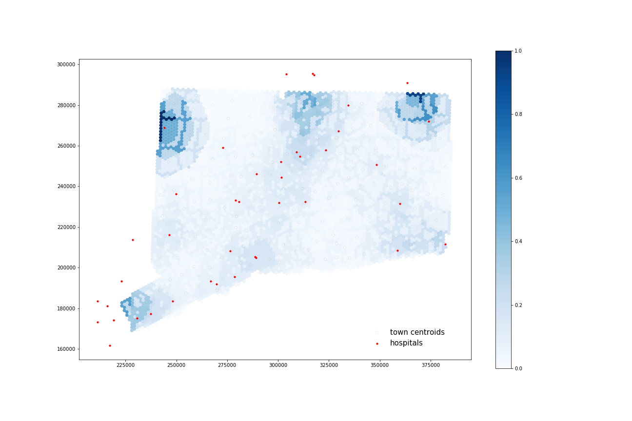
Using four processors, it took 63.119 seconds to calculate 38 catchments and 69.086 seconds to calculate their overlapping areas.
At-Risk Population:
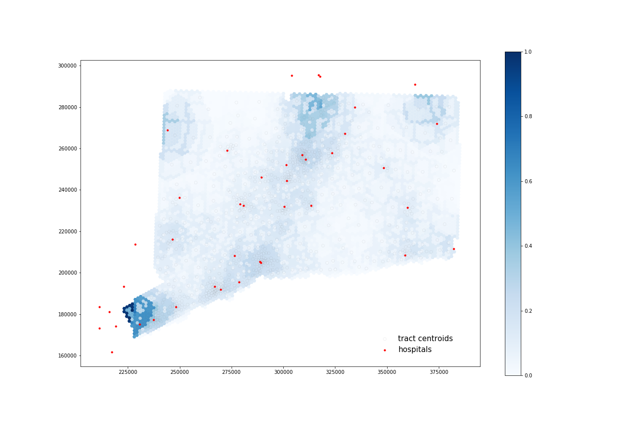
Using four processors, it took 67.942 seconds to calculate 40 catchments and 67.942 seconds to calculate their overlapping areas.
Access to ICU Beds
COVID-19 Patients:
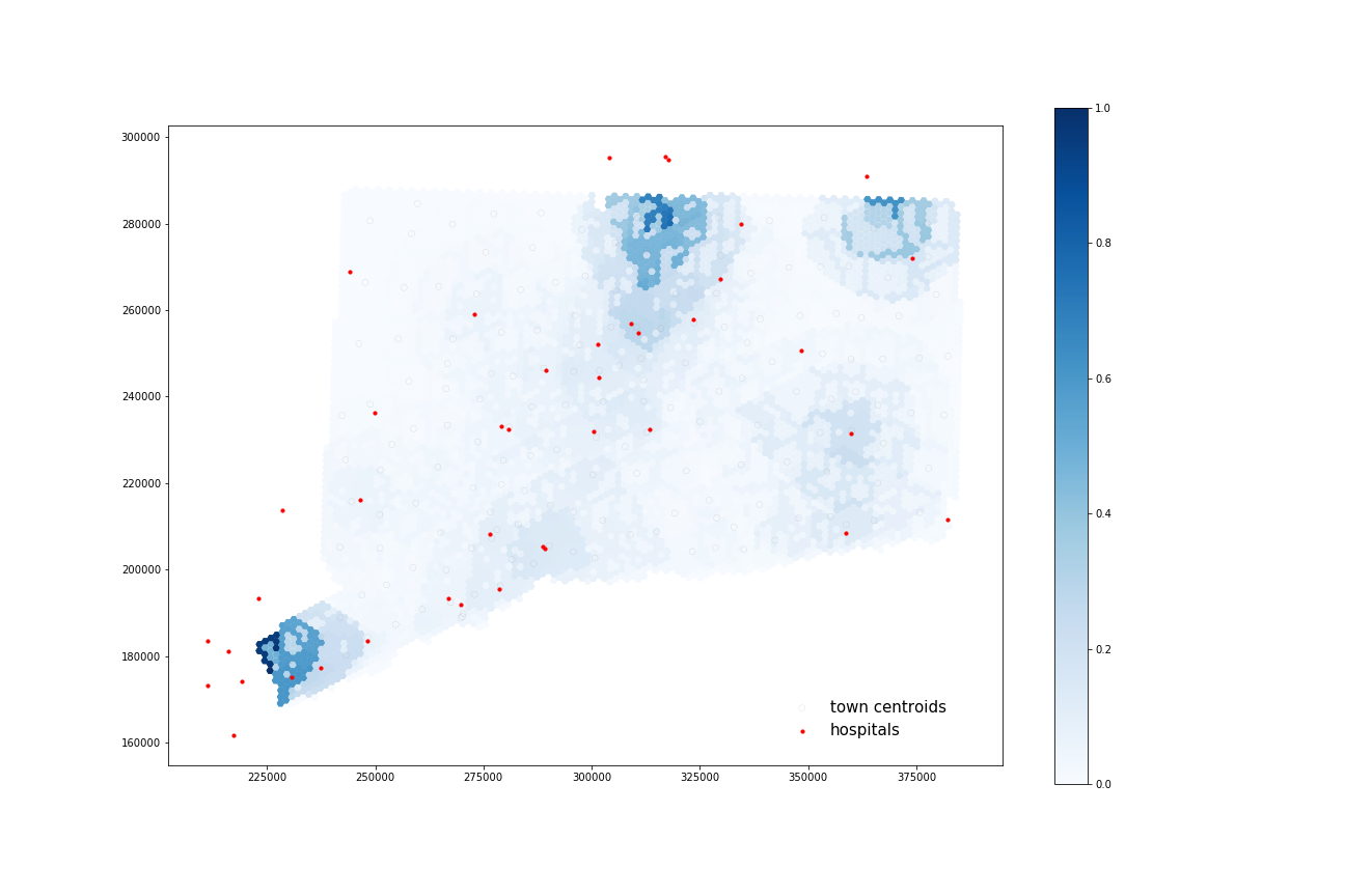
Using four processors, it took 61.103 seconds to calculate 35 catchments and 68.721 seconds to calculate their overlapping areas.
At-Risk Population:
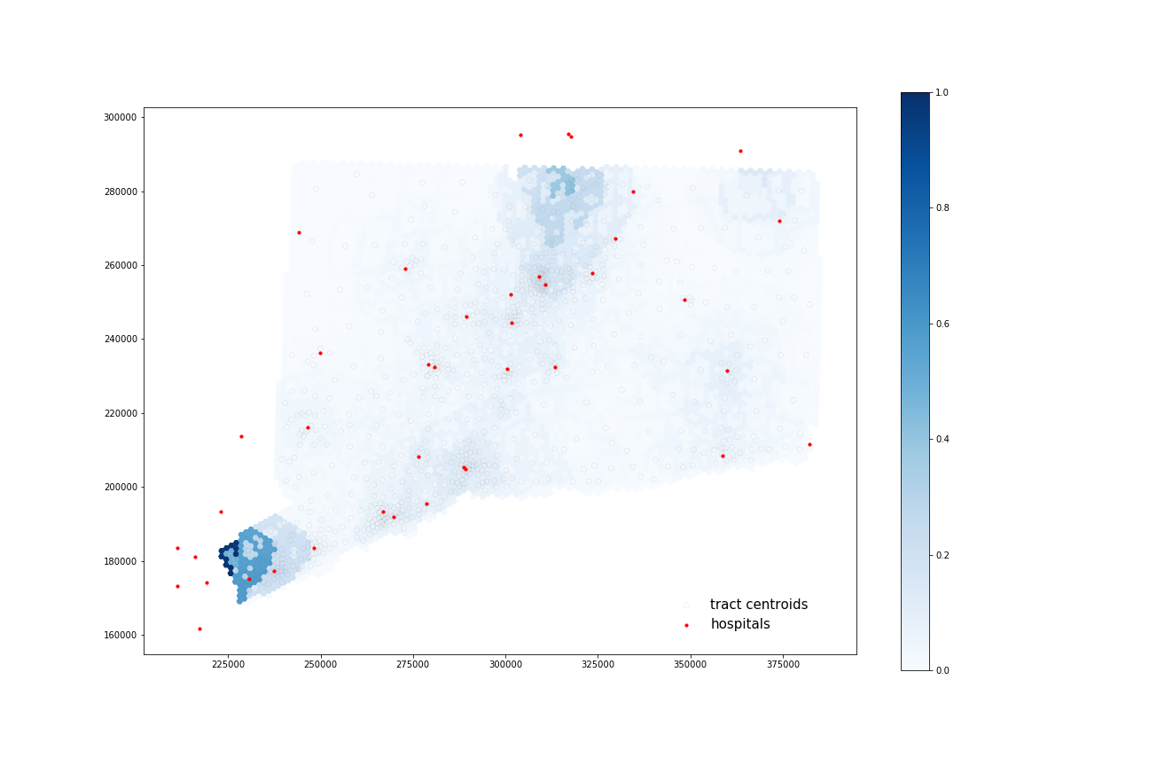
Using four processors, it took 56.078 seconds to calculate 35 catchments and 69.218 seconds to calculate their overlapping areas.
All four maps display some similar geographic distributions, with their highest accessibility ratings in the southeastern portion of the state (near Greenwich, Wesport, New Canaan) and in the north central portion of the state (just north of Hartford and south of Springfield, Mass). These patterns reveal some of the highest accessibility in regions near state borders, indicating that interstate hospitals can severely increase COVID-19 healthcare access for Connecticut residents. All four maps show much lower accessibility levels across all four combinations in the state’s less populated counties: Litchfield, New London, and Windham.
COVID-19 patients appear to have higher accessibility to both general beds and ICU beds compared to the At-Risk population. Their access increases especially in more urban areas of that state (New Haven, Norwalk, and North of Hartford) as well as along border regions near hospitals from other states.
Discussion and Conclusion
Connecticut Spatial Accessibility
In terms of the results from this replication, it is clear that, in mid-November, COVID-19 patients had better access to hospital beds in Connecticut than the at-risk population. This might be explained by a higher presence of COVID-19 cases in these urban areas, where there are higher concentrations of healthcare resources. Additionally, this map of proportion over fifty by tract shows that the at risk population are in some of these lower accessibility areas. If outbreaks increase in some of these less populated regions of the state, it may be difficult for at risk populations to get the care they need.
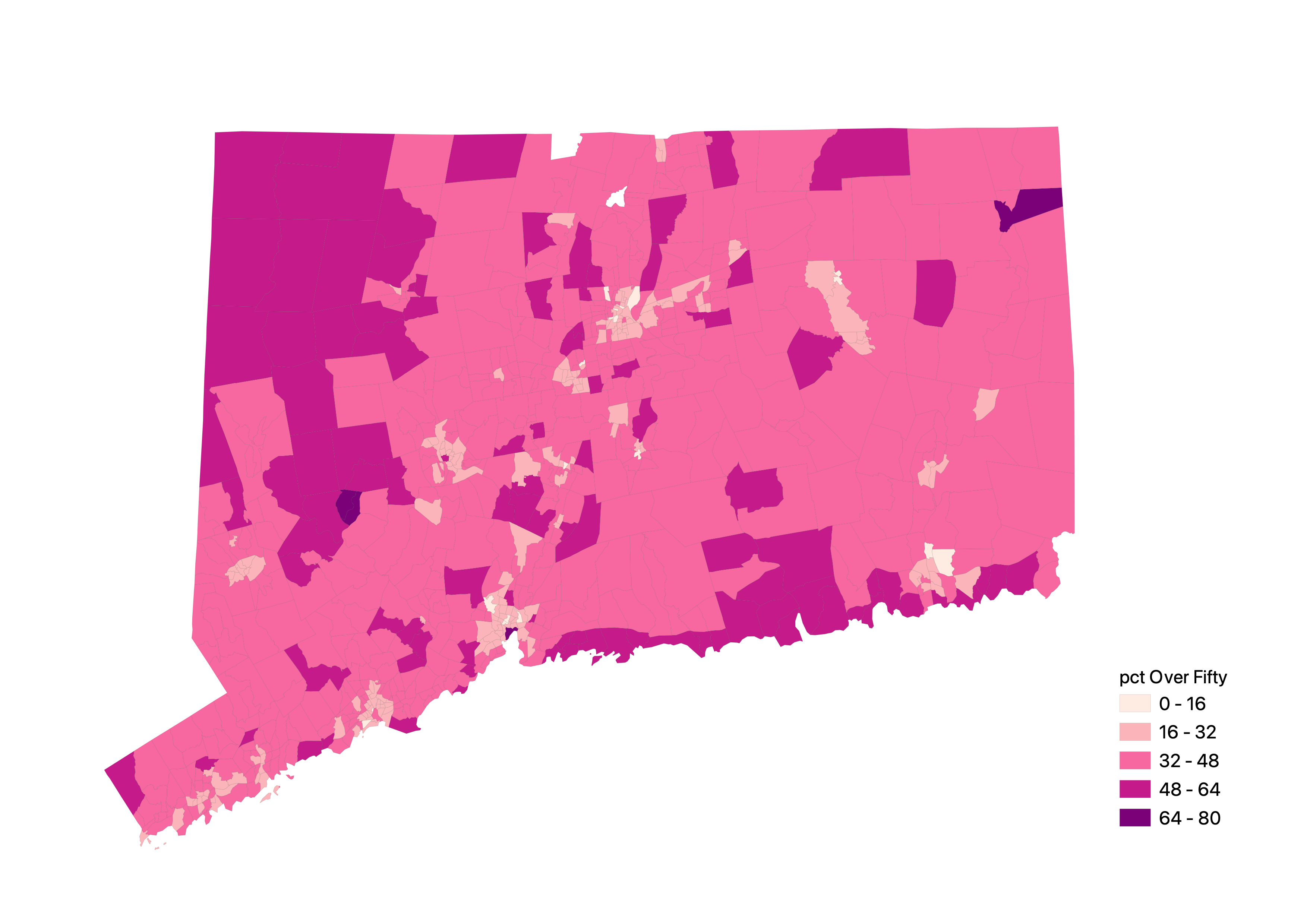
Despite these findings, this analysis operates under the assumption that all of the hospitals across state borders will accept CT patients. Further, the analysis does not take into account the capacity of these hospitals across statelines. Thus, these assumptions have the potential to heavily alter the results, and therefore interstate capacity and admittances should be taken into account in future assessment of interstate COVID-19 healthcare access.
Reflection on Reproducibility and Replicability Kang et al’s methodology
With the combination of the jupyter notebook and the paper, Kang et al. provide all the necessary data, code, and conceptual background to make the results of the paper reproducible (Sui 2014). There are currently a couple of impediments that prevent a full reproduction, however. The biggest difficulty is that the Illinois road network graph is not already provided in the Jupyter notebook, forcing users to load the graph. Both Professor Holler and I tried multiple times to download this network graph, but the kernel would consistently shutdown after about 10 or 12 hours of loading. All of the accessibility measurements (including Chicago - to account for hospital access right outside of Chicago) require this network, so the notebook can’t reproduced if this network doesn’t load. This is could be fixed, however, if the network is pre-loaded onto the Jupyter Notebook’s data folder. It seems, that as long as the loaded Illinois network follows the same exact structure as that used in the original analysis (if the road network changes and osmnx is updated accordingly, the results might change as well), we should be able to derive the same results using the same inputs (National Academies of Sciences, Engineering, and Medicine, 2019). Without all the necessary data, however, we cannot say for sure that this is fully reproducible. The other barrier to reproducing the results from the paper is that the SVI portion of the analysis is not included in the notebook.
In terms of replicating the study, some of the biggest barriers lie outside of the control of the authorship. The CyberGISX platform (as long as one has access to it!) allows users to easily replicate the workflow with Jupyter Notebooks. The difficulty lies in the nature of the hospital resource data and the COVID-19 data. Although I was able to find a centralized dataset on national hospital resources, it lacked the ventilator data that the authors were able to acquire from the IDPH, rendering it impossible to replicate that portion of the analysis. Further, I could not find any publicly available zip-code level data for COVID-19 cases at the state level, and had to settle for town-level data, giving a less precise accessibility measurement than the authors have produced.
Lastly, as an undergraduate with no prior experience using python or jupyter notebooks, the authors do provide a solid platform for accessible replication. In conjunction with the paper, the notebook is set up to give users a strong conceptual understanding of what happens under the hood during the P-E2SFCA calculation. It was, at times, a bit difficult to line up which of the 13 or so functions that are defined were covering which part of the paper. If the code were commented more thoroughly, with the goal of lining up, step-by-step, the code with the paper while considering a novice user, it would make the process of learning the notebook more accessible. However, by providing the users the opportunity to examine the code, we are able to get a really solid sense of the true nature of the analytic processes (Singleton 2016), making it easier to understand which parameters we needed to alter to customize our replication. Overall, as long as users are willing to spend a fair amount of time learning the code and its functions, the notebook and the paper allow for a replicable analysis. Most of the issues of replicability pertain to accessing the same data for different regions, which lie outside of the authors’ control.
Resources:
National Academies of Sciences, Engineering, and Medicine. 2019. Reproducibility and Replicability in Science. Washington, DC: The National Academies Press. doi: https://doi.org/10.17226/25303.
Singleton, D.A., Spielman, S. & C Brundson. 2016. Establishing a framework for Open Geographic Information science. International Journal of Geographical Information Science 30(8); 1507-1521. http://dx.doi.org/10.1080/13658816.2015.1137579
Sui, D. 2014. Opportunities and impediments for Open GIS. Transactions in GIS, 18(1); 1-24. doi:10.1111/tgis.12075